Gaussian graphical models with skggm

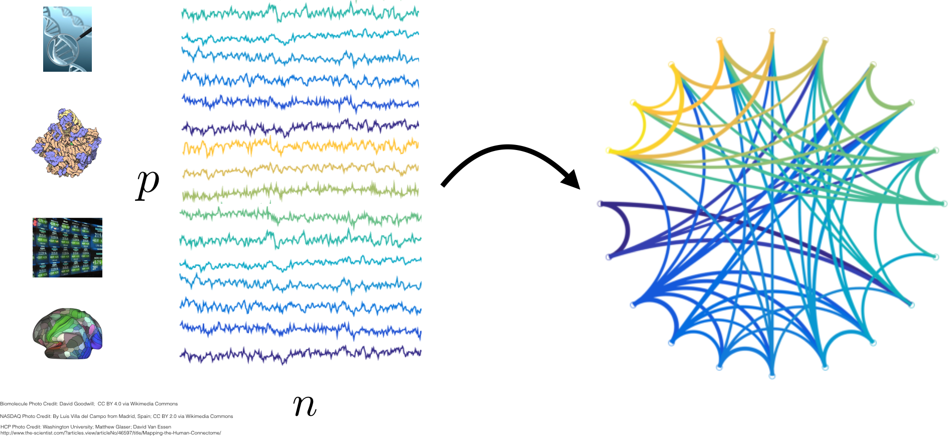
Graphical models combine graph theory and probability theory to create networks that model complex probabilistic relationships. Inferring such networks is a statistical problem in areas such as systems biology, neuroscience, psychometrics, and finance.

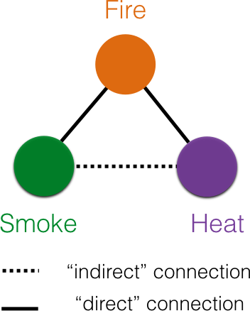
A simple model to infer a network between $p$ variables is a correlational network. In this case, if two variables are correlated, then the corresponding nodes are connected by an edge, but not otherwise. Thus the absence of an edge between two nodes indicates the absence of a correlation between them. Unfortunately, as shown in Figure 2, such pairwise correlations could be spuriously induced by shared common causes.

Thus, in applications that seek to interpret edges as some form of direct influence, more sophisticated graphical models that eliminate spurious or misleading relationships are desirable. This motivates the usage of Markov networks, popularly known as Gaussian graphical models for Gaussian distributed data. First, we briefly introduce the notion of Markov networks for general probability distributions before considering the case of multivariate Gaussians. Then, we consider a particularly efficient way to estimate Gaussian graphical models via the inverse covariance. Last, but not least, we lay out how skggm implements a variety of important maximum likelihood estimators for the inverse covariance.

• Conditional independence and Markov networks
• Markov networks and inverse covariance
• Maximum likelihood estimators
• A tour of skggm: methods & interfaces
  • Model selection via cross-validation (less sparse)
  • Model selection via EBIC (more sparse)
  • Randomized model averaging
  • Refining estimates via adaptive methods
• Discussion

Conditional independence and Markov networks

Formally, a graph $\mathcal{G}=(V,E)$ consists a set of vertices $V = \{1,\ldots,p\}$ and edges between them $E\subset V \times V$. The vertices or nodes are associated with a $p$-dimensional random variable $\Xdata = (X_{1},\ldots, X_{p})$ that has some probability distribution $\Xdata \sim \mathbb{P}_{\Xdata}$.

There are many probabilistic graphical models that relate the structure in the graph $\mathcal{G}$ to the probability distribution over the variables $\mathbb{P}_{\Xdata}$. We discuss an important class of graphical models, Markov networks, that relate absence of edges in the graph to conditional independence between random variables $X_{1},\ldots, X_{p}$. A particular graph $\mathcal{G}$ and probability distribution $\mathbb{P}_{\Xdata}$ forms a Markov network if it satisfies one of the Markov properties:

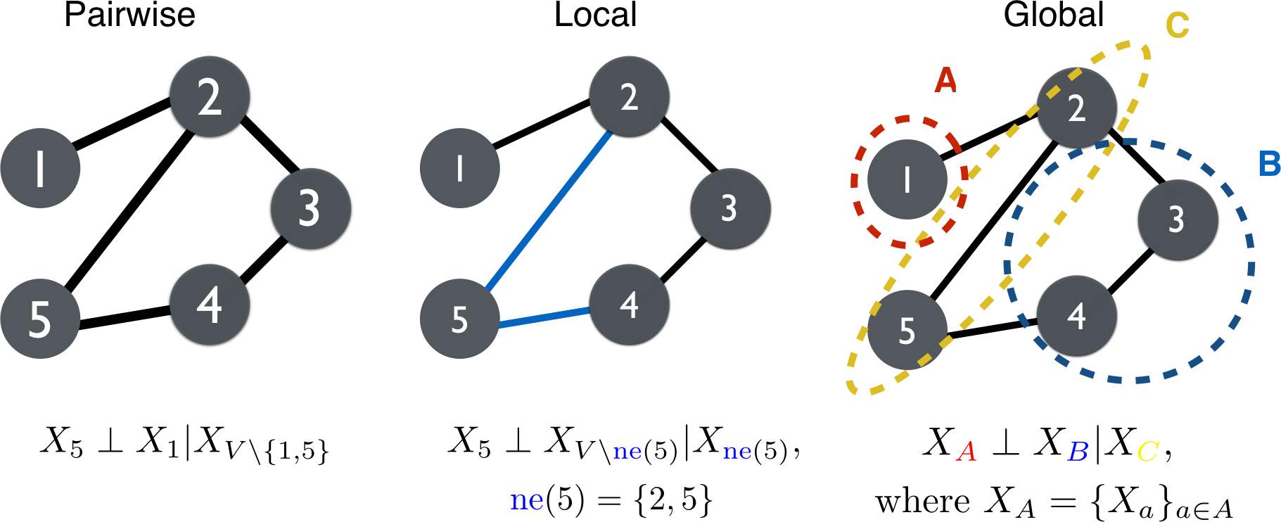
We denote statistical independence by $\perp$ and conditioning by $\mid$. The properties depicted in Figure 3 are as follows.

1. Pairwise: The absence of an edge $(j,k) \not\in E$ implies

   $$\begin{align} \label{eqn:pairwise} X_{j} \perp X_{k} | \ X_{V \setminus \{j,k\}}, \quad \forall \ j \in V, ~k \in V, ~j \ne k.\tag{$\textbf{P}$} \end{align}$$

2. Local: Given $j \in V$ and its neighbors $ne(j)$,

   $$\begin{align} \label{eqn:local} X_{j} \perp X_{V \setminus \{j,\text{ne}(j)\}} | \ X_{ne(j)}, \quad \forall j \in V\tag{$\textbf{L}$} \end{align}$$

   where $ne(j) = \{k \in V: (j,k) \in E, \ j \ne k \}$.

3. Global: All paths between $A$ and $B$ are separated by $C$ implies

   $$\begin{align} \label{eqn:global} X_{A} \perp X_{B} | \ X_{C}\tag{$\textbf{G}$} \end{align}$$

   for all disjoint subsets $A,B,C \subset V$, where $C$ separates $A$ and $B$.

The pairwise Markov property is the weakest Markov property while the global Markov property is the strongest. If a distribution satisfies the global property it implies all the others, i.e., $(\ref{eqn:global}) \Rightarrow (\ref{eqn:local}) \Rightarrow (\ref{eqn:pairwise})$. For some special distributions that have positive densities such as the multivariate Gaussian, the compositional property of conditional independence holds. As a result, $(\ref{eqn:pairwise}) \Rightarrow (\ref{eqn:global})$ and all three Markov properties are equivalent. Typically, the term Markov networks refers to networks that satisfy (\ref{eqn:global}), otherwise they might be called local or pairwise Markov networks depending on the strongest property satisfied.

When probability distributions satisfy the global Markov property, it becomes computationally and statistically tractable to efficiently infer conditional independence relationships. For an extensive reference on Markov properties of directed and undirected Markov networks, please see “Graphical Models” by Lauritzen.

Markov networks and inverse covariance

If two variables are statistically independent they are also uncorrelated, however, the converse is not necesssarily true. Since Gaussian distributions are fully described by their mean and covariance, a zero correlation between two variables also implies statistical independence. An analogous equivalence holds between conditional independence and the inverse covariance for Gaussian distributions.

Given $n$ i.i.d random samples $(x_{1},x_{2},\ldots,x_{n})^{\top} = \Xdata$ from a multivariate Gaussian distribution

where each sample $x_{i} \in \mathbb{R}^{p}$ is $p$-dimensional, and $\Sig$ is the population covariance matrix $\Sig = \mathbf{E}(\Xdata^{\top}\Xdata)$. We denote the inverse covariance by $\Thet = \Sig^{-1}$.

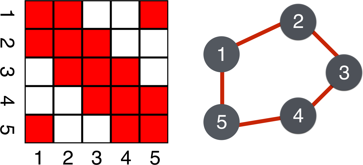
As a consequence of the Hammersley-Clifford theorem in the case of Gaussian distributions, $\Thet_{jk} = 0 \iff (j,k) \not \in E \iff X_{j} \perp X_{k} \mid \ X_{V \setminus \{j,k\}}$. Thus, as shown in Figure 4, a zero in the inverse covariance is equivalent to conditional independence and the absence of an edge in the graph. Furthermore, partial correlations are proportional to entries of the inverse covariance and thus this property also holds for the partial correlation matrices.

The inverse covariance matrix is an important quantity of interest as it gives us an efficient way of obtaining the structure of the Markov network. The lasso regularized maximum likelihood estimator, otherwise known as the graphical lasso (\ref{eqn:graphlasso}) explained below, is a popular statistical method for estimating such inverse covariances from high dimensional data. In the python package skggm we provide a scikit-learn-compatible implementation of the graphical lasso and a collection of modern best practices for working with the graphical lasso and its variants.

The concept of Markov networks has been extended to many other measures of association beyond the standard covariance. These include covariances between variables in the Fourier domain (cross-spectral density) encountered in time-series analyses and information theoretic measures. Moreover, for some non-Gaussian distributions, zeros in a generalized inverse covariance can provide conditional independence relationships analogous to standard inverse covariance explained above. Given the general importance of the inverse covariance, we expect methods for estimating it to be useful for many other classes of graphical models beyond standard Gaussian graphical models. Thus, while skggm currently supports standard inverse covariances for multivariate normal distributions, we hope this implementation will serve as a foundational building block for generalized classes of graphical models.

Maximum likelihood estimators

The maximum likelihood estimate of the precison

can be computed via the sample covariance given by $\hat{\Sig} = \frac{1}{n - 1} \sum_{i=1}^{n} (x_{i} - \bar{x}) (x_{i} - \bar{x})^{\top}$ for samples $\{x_{j}\}$ and sample mean $\bar{x}$. To ensure all features are on the same scale, sometimes the sample covariance is replaced by the sample correlation $\mathbf{R}(\hat{\Sig})$ using the variance-correlation decomposition $\mathbf{R}(\hat{\Sig}) = \hat{\mathbf{D}}\ \hat{\Sig}\ \hat{\mathbf{D}}$, where the diagonal matrix, $\hat{\mathbf{D}}=\text{diag}(\hat{\sigma}^{-1/2}_{11},\ldots,\hat{\sigma}^{-1/2}_{pp})$, is a function of the sample variances from $\hat{\Sig}$.

When the number of available samples $n$ are fewer than or comparable to the number of variables $n \le p$, the sample covariance becomes ill-conditioned and finally degenerate. Consequently taking its inverse and estimating up to $\frac{p(p-1)}{2}$ off-diagonal coefficients in the inverse covariance becomes difficult. To address the degeneracy of the sample covariance and the likelihood (\ref{eqn:mle}) in high dimensions, many including Yuan and Lin, Bannerjee et al., and Friedman et al. proposed regularizing maximum likelihood estimators with sparsity-enforcing penalties such as the lasso. Sparsity-enforcing penalties assume that many entries in the inverse covariance will be zero. Thus fewer than $\frac{p(p-1)}{2}$ parameters need to be estimated, though the location of these non-zero parameters is unknown. The lasso regularized MLE objective is given by

$\begin{align} \hat{\Thet}(\Lambda) = \underset{\Theta \succ 0}{\mathrm{arg\,min}}~ -\mathrm{log\,det}~\Thet + \mathrm{tr}(\hat{\Sig}\Thet) + \|\Thet\|_{1, \Lambda} \label{eqn:graphlasso}\tag{2} \end{align}$ where $\Lambda$ is a $p \times p$ symmetric matrix with non-negative entries and $\|\Thet\|_{1, \Lambda} = \sum_{j,k=1}^{p} \lambda_{jk}\mid\theta_{jk}\mid$. Typically, we avoid penalizing the diagonals by setting $\lambda_{jj} = 0,\ j=1,\ldots,p$ to ensure that $\hat{\Thet}$ remains positive definite. The objective (\ref{eqn:graphlasso}) reduces to the standard graphical lasso formulation of Friedman et al. when all off diagonals of the penalty matrix take a constant scalar value $\lambda_{jk} = \lambda_{kj} = \lambda$ for all $j \ne k$. The standard graphical lasso has been implemented in scikit-learn.

A tour of skggm: methods & interfaces

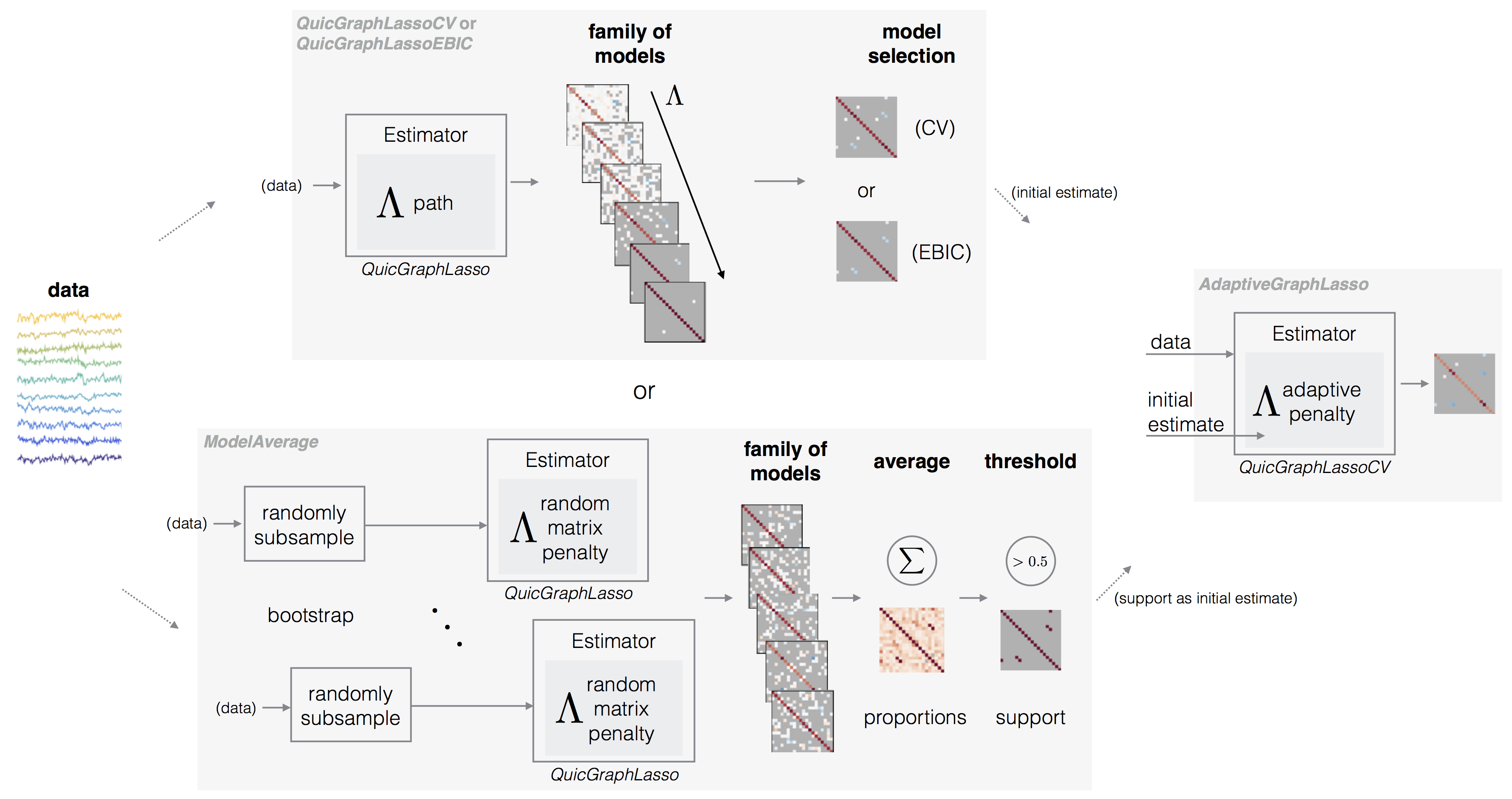
The core estimator provided in skggm is QuicGraphLasso which is a scikit-learn compatible interface to QUIC, a proximal Newton-type algorithm that solves the graphical lasso (\ref{eqn:graphlasso}) objective.

from inverse_covariance import QuicGraphLasso

model = QuicGraphLasso(
    lam=int or np.ndarray,  # Graphical lasso penalty (scalar or matrix) 
    mode=str,               # 'default': single estimate
                            # 'path': use sequence of scaled penalties 
    path=list,              # Sequence of penalty scales mode='path'
    init_method=str,        # Initial covariance estimate: 'corrcoef' or 'cov'
    auto_scale=bool,        # If True, scales penalty by 
                            # max off-diagonal entry of the sample covariance
)
model.fit(X)                # X is data matrix (n_samples, n_features) 

If the input penalty lam is a scalar, it will be converted to a matrix with zeros along the diagonal and lam for all other entries. A matrix lam is used as-is, although it will be scaled if auto_scale=True.

After the model is fit, the estimator object will contain the covariance estimate model.covariance_ $\in \mathbb{R}^{p\times p}$, the sparse inverse covariance estimate model.precision_ $\in \mathbb{R}^{p\times p}$, and the penalty model.lam_ used to obtain these estimates. When auto_scale=False, the output pentalty will be identical to the input penalty. If mode='path' is used, then the path parameter must be provided and both model.covariance_ and model.precision_ will be a list of $p\times p$ matrices of length len(path). In general, the estimators introduced here will follow this interface unless otherwise noted.

The graphical lasso (\ref{eqn:graphlasso}) provides a family of estimates $\Thet(\Lambda)$ indexed by the regularization parameter $\Lambda$. The choice of the penalty $\Lambda$ can have a large impact on the kind of result obtained. If a good $\Lambda$ is known a priori, e.g., when reproducing existing results from the literature, then look no further than this estimator (with auto_scale='False'). Otherwise when $\Lambda$ is unknown, we provide several methods for selecting an appropriate $\Lambda$. Selection methods roughly fall into two categories of performance: a) overselection (less sparse), resulting in estimates with false positive edges; or b) underselection (more sparse), resulting in estimates with false negative edges.

Model selection via cross-validation (less sparse)

A common method to choose $\Lambda$ is cross-validation. Specifically, given a grid of penalties and K folds of the data,

1. Estimate a family of sparse to dense precision matrices on $K-1$ folds of the data.
2. Score the performance of these estimates on the $K^{\text{th}}$ fold using some loss function.
3. Repeat Steps 1 and 2 over all folds.
4. Aggregate the score across the folds in Step 3 to determine a mean score for each $\Lambda$.
5. Pick the value of $\Lambda$ that minimizes the mean score.

We provide several metrics of the form $d(\hat{\Sig}, \hat{\Thet})$ that measure how well the inverse covariance estimate fits the data. These metrics can be combined with cross-validation via the score_metric parameter. Since CV measures out-of-sample error, we estimate inverse covariance $\hat{\Thet}$ on the training set and measure its fit against the sample covariance $\hat{\Sig}$ on the test set. The skggm package offers the following options for the CV-loss, $d(\hat{\Sig}^{ts},\hat{\Thet}^{tr})$:

Cross validation can be performed with QuicGraphLasso and GridSearchCV, however, we provide an optimized convenience class QuicGraphLassoCV that takes advantage of path mode to adaptively estimate the search grid. This implementation is closely modeled after scikit-learn’s GraphLassoCV, but with support for matrix penalties.

from inverse_covariance import QuicGraphLassoCV

model = QuicGraphLassoCV(
    lam=int or np.ndarray,  # (optional) Initial penalty (scalar or matrix) 
    lams=int or list,       # If int, determines the number of grid points 
                            # per refinement
    n_refinements=int,      # Number of times the grid is refined
    cv=int,                 # Number of folds or sklearn CV object
    score_metric=str,       # One of 'log_likelihood' (default), 'frobenius', 
                            #        'kl', or 'quadratic'
    init_method=str,        # Initial covariance estimate: 'corrcoef' or 'cov'
)
model.fit(X)                # X is data matrix (n_samples, n_features) 

In addition to covariance and precision estimates, this class returns the best penalty in model.lam_ and the penalty grid model.cv_lams_ as well as the cross-validation scores for each penalty model.grid_scores.

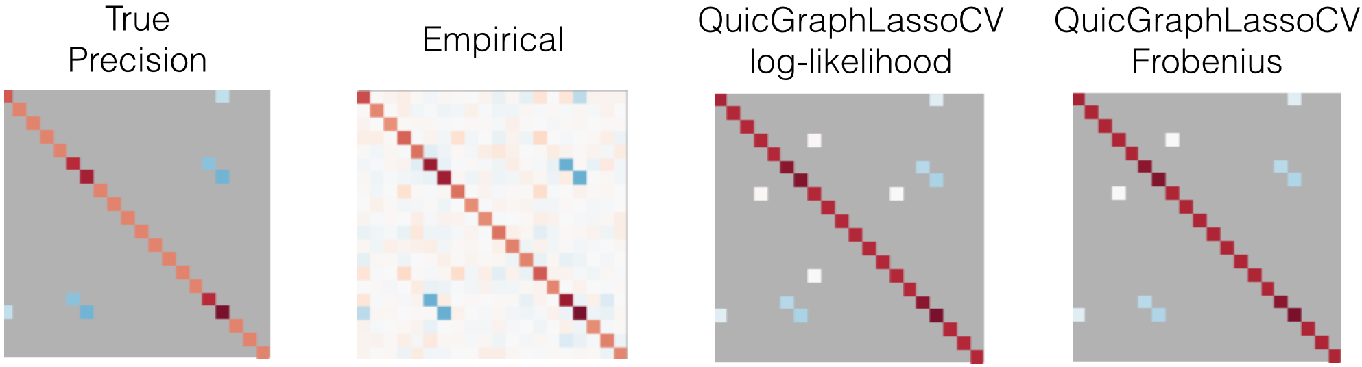
An example is shown in Figure 6. The QuicGraphLassoCV estimates are much sparser than the empirical precision, but are a superset of the true precision support. As the dimension of the samples n_features grows, we find that this model selection method tends to bias toward more non-zero coefficients. Further, the coefficient values on the true support are not particularly accurate.

In this trial of this example, the Frobenius scoring function performed better than log-likelihood and KL-divergence, however, this does not reflect how they might compare with different underlying networks and/or in larger dimensions.

Code for the example above and those that follow can be found in skggm in examples/estimator_suite.py.

Model selection via EBIC (more sparse)

An alternative to cross-validation is the Extended Bayesian Information Criteria (EBIC) [Foygel et al.],

where $\mathcal{L}(\hat{\Thet}, \hat{\Sig})$ denotes the log-likelihood (\ref{eqn:mle}) between the estimate and the sample covariance, and $\mid\hat{E}(\hat{\Thet}(\lambda))\mid$ denotes number of estimated edges or non-zeros in $\hat{\Thet}(\lambda)$. The parameter $\gamma$ can be used to choose sparser graphs for higher dimension problems $p>>n$. When $\gamma = 0$, the EBIC criterion (\ref{eqn:ebic}) reduces to the conventional Schwarz or Bayesian information crieteria (BIC).

QuicGraphLassoEBIC is provided as a convenience class to use EBIC for model selection. This class computes a path of estimates and selects the model that minimizes the EBIC criteria. We omit showing the interface here as it is similar to the classes described above with the addition of the gamma.

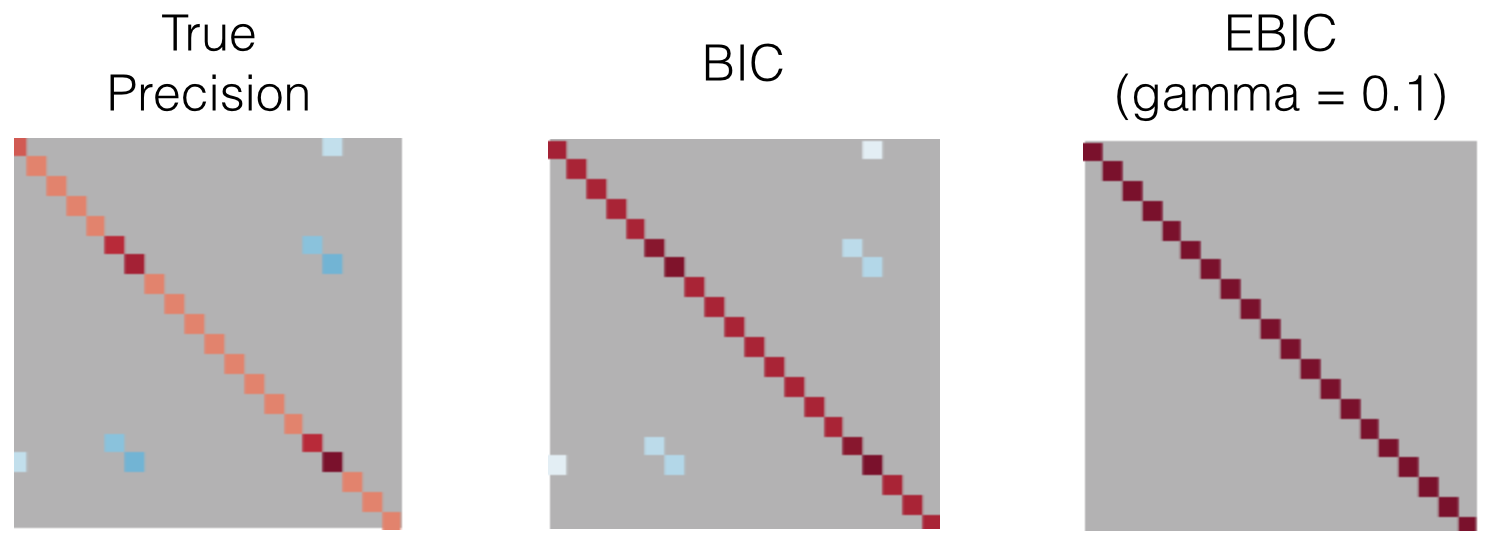
An example is shown in Figure 7. The QuicGraphLassoEBIC estimates are much sparser than QuicGraphLassoCV estimates, and often contain a subset of the true precision support. In this small dimensional example, BIC (gamma = 0) performed best, as EBIC with gamma = 0.1 selected only the diagonal coefficients. As the dimension of the samples n_features grows, BIC will select a less-sparse result and thus an increasing gamma parameter serves to obtain sparser solutions.

Randomized model averaging

For some problems, the support of the sparse precision matrix is of primary interest. In these cases, the true support can be estimated with greater confidence by employing a form of ensemble model averaging known as stability selection [Meinhausen et al.] combined with randomizing the model selection via the random lasso [Meinhausen et al., Wang et al.]. The skggm ModelAverage class implements a meta-estimator to do this. This is a similar facility to scikit-learn’s RandomizedLasso but for the graphical lasso.

This technique estimates the precision over an ensemble of estimators with random penalties and bootstrapped samples. Specifically, in each trial we

1. Draw boostrap samples by randomly subsampling $\Xdata$.
2. Draw a random matrix penalty.

A final proportion matrix is then estimated by summing or averaging the precision estimates from each trial. The precision support can be estimated by thresholding the proportion matrix.

The random penalty can be chosen in a variety of ways. We initially offer the following methods:

• subsampling (fixed penalty): This option does not modify the penalty and only draws bootstrapped samples from $\Xdata$. Use this in conjunction with a scalar penalty.

• random: This option generates a randomly perturbed penalty weight matrix. Specifically, the off-diagonal entries take the values $\{\lambda\eta,~ \frac{\lambda}{\eta}\}$ with probability $1/2$. The class uses lam_perturb for $\eta$.

• fully_random: This option generates a symmetric matrix with Gaussian off-diagonal entries (for a single triangle). The penalty matrix is scaled appropriately for $\Xdata$.

ModelAverage takes the parameter estimator as the graphical lasso estimator instance to build the ensemble and by default, QuicGraphLassoCV is used.

from inverse_covariance import ModelAverage

model = ModelAverage(
    estimator=estimator,    # Graphical lasso estimator instance 
                            # e.g., QuicGraphLassoCV(), QuicGraphLassoEBIC()
    n_trials=int,           # Number of trials to average over
    penalization=str,       # One of 'subsampling', 'random' (default), 
                            #        or 'fully_random'
    lam=float,              # Used if penalization='random'          
    lam_perturb=float,      # Used if penalization='random'
    support_thresh=float,   # Estimate support via proportions (default=0.5)
)
model.fit(X)                # X is data matrix (n_samples, n_features)             

This class will contain the matrix of support probabilities model.proportion_ $\in \mathbb{R}^{p\times p}$, an estimate of the support model.support_ $\in \mathbb{R}^{p\times p}$, the penalties used in each trial model.lams_, and the indices for selecting the subset of data in each trial model.subsets_.

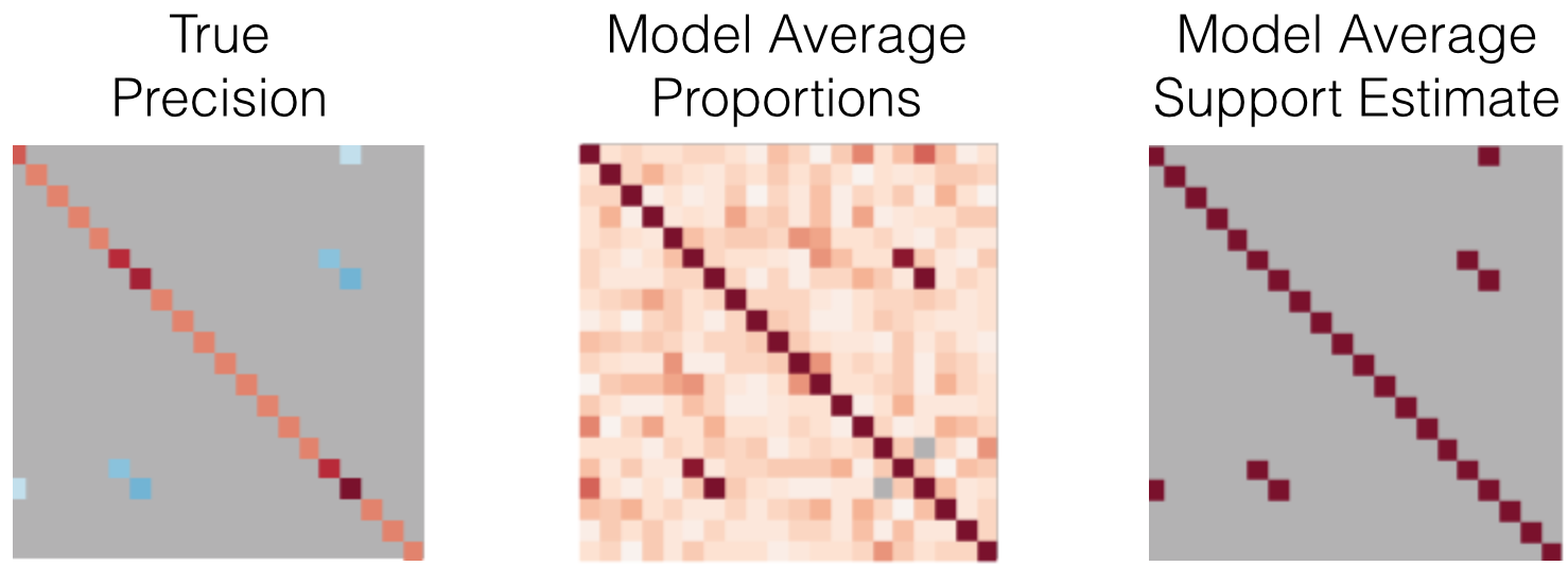
An example is shown in Figure 8. The dense model.proportions_ matrix contains the sample probability of each element containing a nonzero. Thresholding this matrix by the default value of 0.5 resulted in a correct estimate of the support. This technique generally provides a more robust support estimate than the previously explained methods. One drawback of this approach is the significant time-cost of running the estimator over many trials, however these trials are easily parallelized.

Refining estimates via adaptive methods

Given an initial sparse estimate, we can derive a new “adaptive” penalty and refit the graphical lasso using data dependent weights $W$ [Zhou et al., Meinhausen et al.]. Thus, the adaptive variant of the graphical lasso (\ref{eqn:graphlasso}) amounts to

In our current implementation, refitting is always done with QuicGraphLassoCV. We provide three ways of computing new weights in (\ref{eqn:adaptive-weights}) before refitting, given the coefficients $\hat{\theta}_{jk}$ of the inverse covariance estimate $\hat{\Thet}$:

• binary: The weight $W_{jk} = 0$ is zero where the estimated entry $\hat{\theta}_{jk} \ne 0$ is non-zero, otherwise the weight is $W_{jk} = 1$. This is sometimes called the refitted MLE or gelato, and similar to relaxed lasso.

• inverse: The weight $W_{jk}$ is set to $\frac{1}{\mid\hat{\theta}_{jk}\mid}$ for non-zero coefficients and $\mathrm{max}\left\{\frac{1}{\hat{\theta}_{jk}}\right\}$ for the zero valued coefficients. This is the default method in the adaptive lasso and in the glasso R package.

• inverse_squared: The weight $W_{jk}$ is set to $\frac{1}{\hat{\theta}_{jk}^{2}}$ for non-zero coefficients and $\mathrm{max}\left\{\frac{1}{\hat{\theta}_{jk}^{2}}\right\}$ for the zero valued coefficients.

Since the ModelAverage meta-estimator produces a good support estimate, this can be combined with the binary option for the weights to combine adaptivity and model averaging.

from inverse_covariance import AdaptiveGraphLasso

model = AdaptiveGraphLasso(
    estimator=estimator,    # Graph lasso estimator instance
                            # e.g., QuicGraphLassoCV() or QuicGraphLassoEBIC()
                            #       or ModelAverage()
    method=str,             # One of 'binary', 'inverse', or 'inverse_squared'
)
model.fit(X)                # X is data matrix (n_samples, n_features)            

The resulting model will contain model.estimator_ which is a final QuicGraphLassoCV instance fit with the adaptive penalty model.lam_.

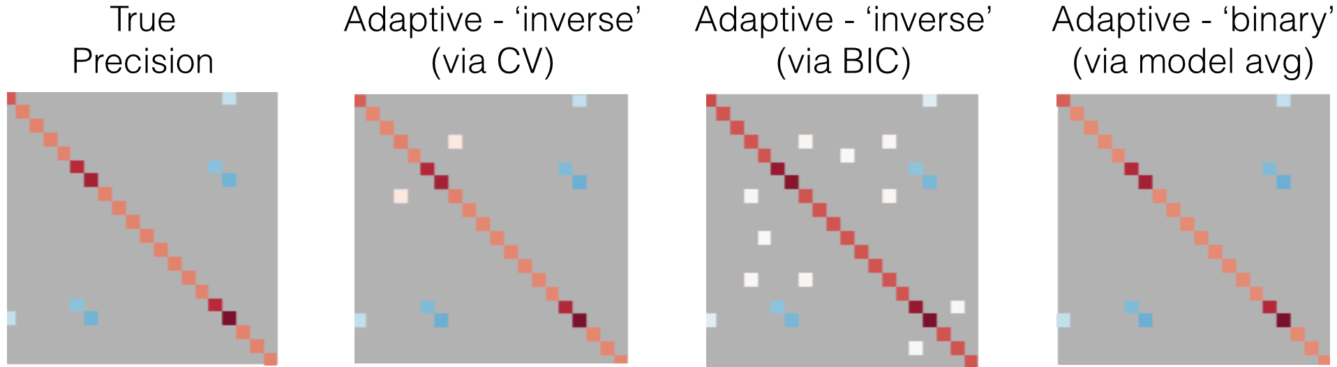
An example is shown in Figure 9. The adaptive estimator will not only refine the estimated coefficients but also produce a new support estimate. This can be seen in the example as the adaptive cross-validation estimator produces a smaller support than the adaptive BIC estimator, the opposite of what we found in the non-adaptive examples.

It is clear that the estimated values of the true support are much more accurate for each method combination. For example, even though the support error for BIC is 10 as opposed to 0 in the non-adaptive case, the Frobenius error is 0.38 while it was 0.68 in the non-adaptive case.

Discussion

In this post, we’ve briefly overviewed the relationship between Markov networks and inverse covariance, discussed estimation via the graphical lasso, and toured through some of the core features of the first release of skggm. We have additional jupyter notebooks and accompanying slides that work through inverse covariance estimation for more difficult network structures.

The following chart depicts the various features supported in skggm and contrasts this with currently available tools for scikit-learn.

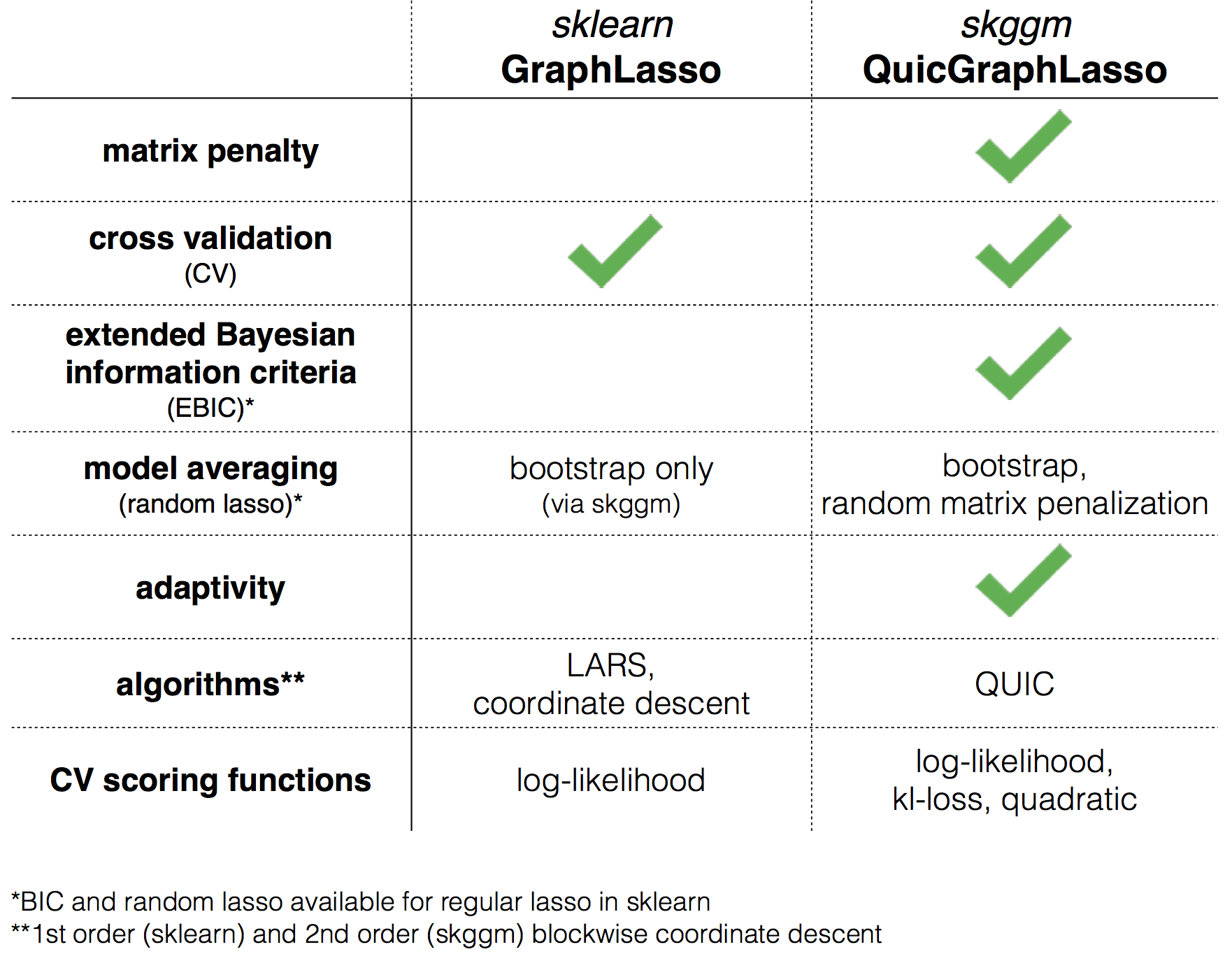
Development of skggm is an ongoing effort. We’d love your feedback on which algorithms and techniques we should include and how you’re using the package. We also welcome contributions.

Acknowledgements: The authors would like to thank Jason Crawford for reading drafts of this post and providing feedback. Some introductory material and figures have been adapted from @mnarayan’s dissertation.

@jasonlaska and @mnarayan, October 10, 2016.

This work is licensed under a Creative Commons Attribution 4.0 International License.